Data
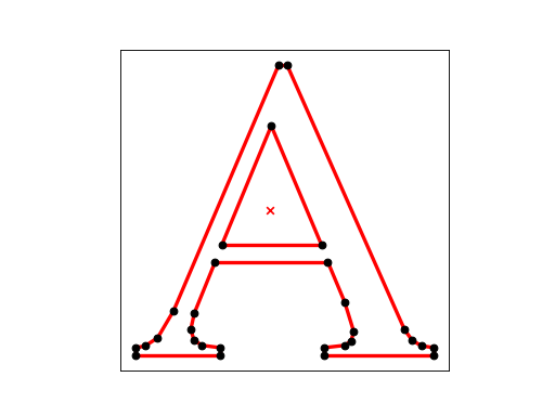
A
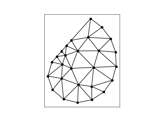
A is a planar straight line graph of the capital letter A. We use it as input to get a constrained Delaunay triangulation.
(Source code, png, hires.png, pdf)
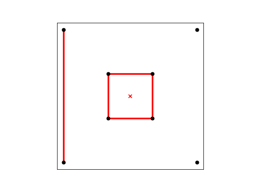
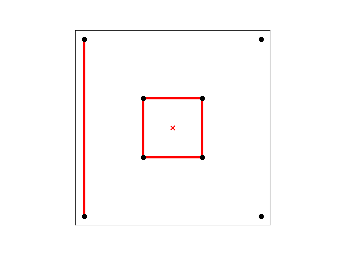
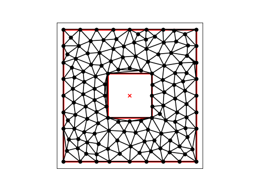
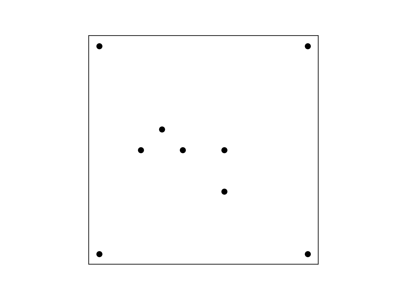
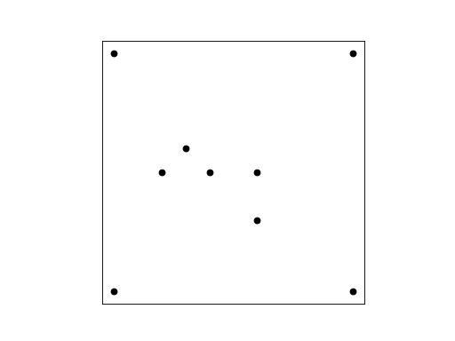
BOX
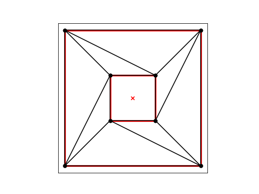
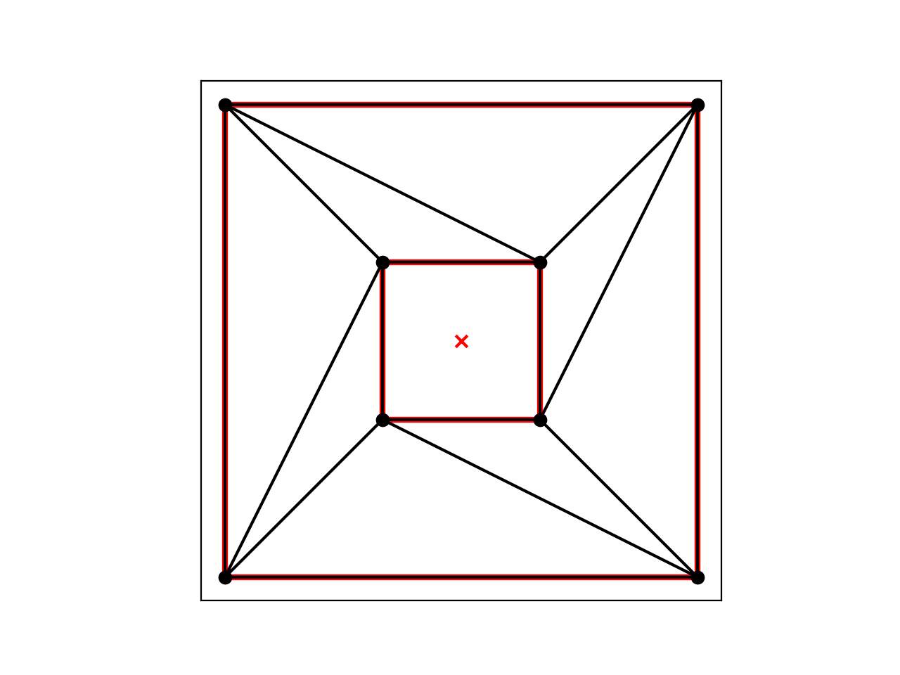
BOX is a planar straight line graph of a double box. We use it as input to get a constrained Delaunay triangulation.
(Source code, png, hires.png, pdf)

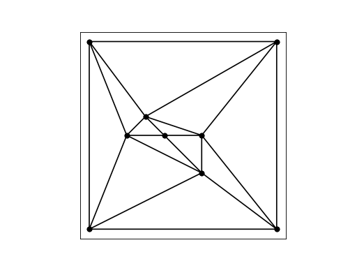
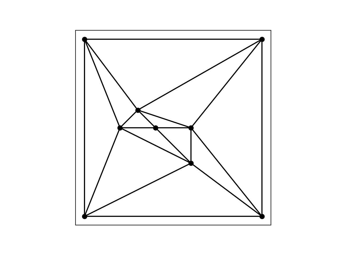
The command:
triangulate(box, opts='pc')
creates the first mesh. (We need the pc because we didn’t surround our initial area with segments.)
(Source code, png, hires.png, pdf)

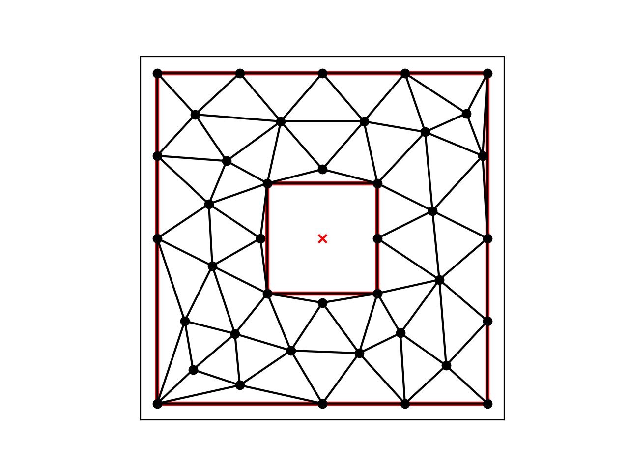
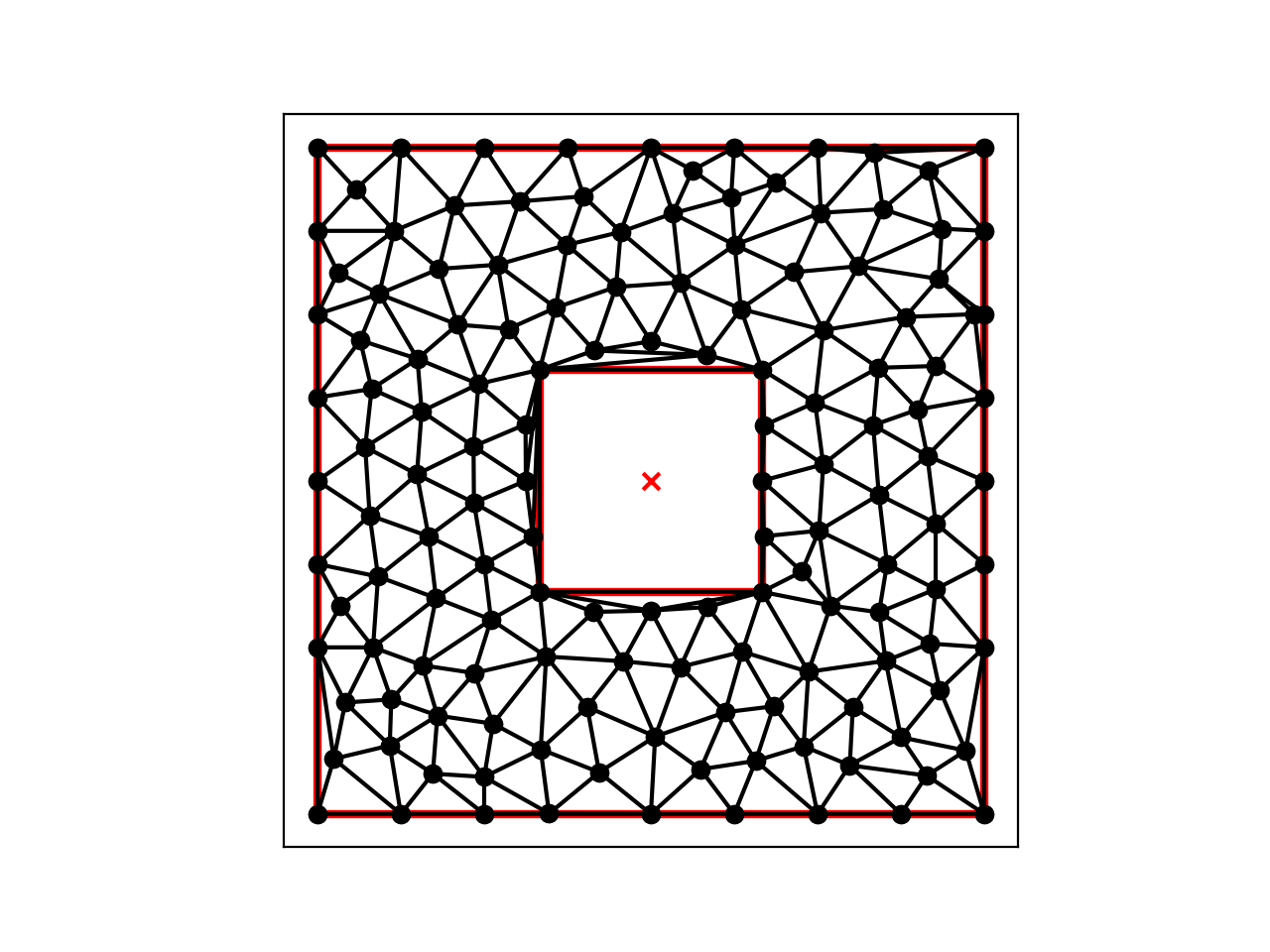
The command:
box1 = get_data('box.1')
triangulate(box1, opts='rpa0.2')
refines the box.1 mesh with an area constraint of 0.2:
(Source code, png, hires.png, pdf)
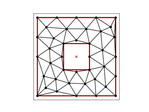
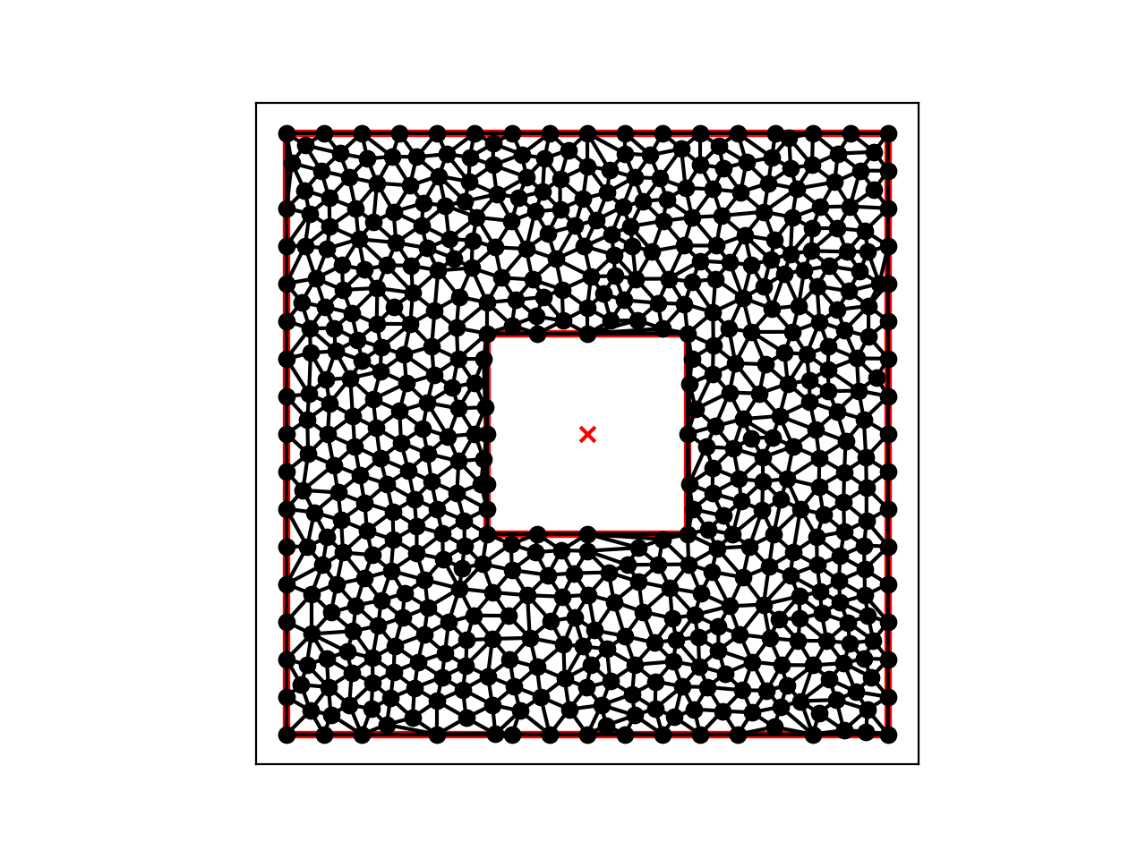
The command:
box2 = get_data('box.2')
triangulate(box2, opts='rpa0.05')
refines the box.2 mesh with an area constraint of 0.05, 1/4 of the previous maximum area:
(Source code, png, hires.png, pdf)

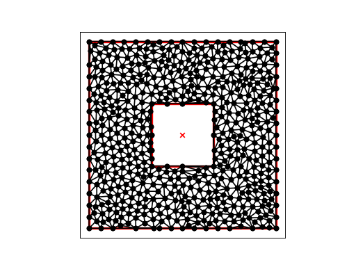
The command “triangulate(box3, opts=’rpa0.0125’)” refines the box.3 mesh with an area constraint of 0.0125, 1/4 of the previous maximum area:
(Source code, png, hires.png, pdf)
DIAMOND_02_00009
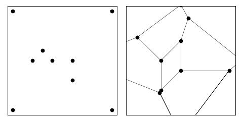
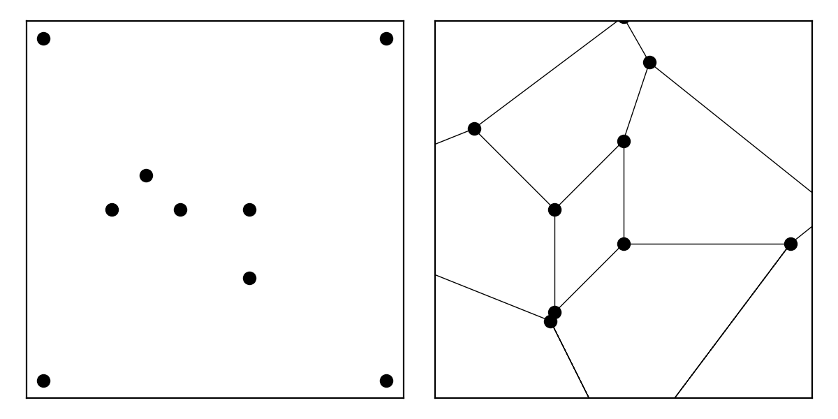
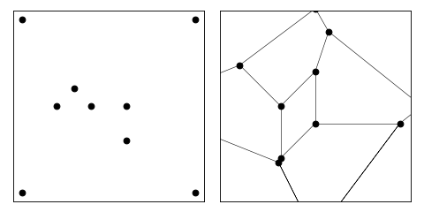
DIAMOND_02_00009 is another set of test data, for which we want the Voronoi diagram.
(Source code, png, hires.png, pdf)
(Source code, png, hires.png, pdf)

(Source code, png, hires.png, pdf)
DOUBLE_HEX
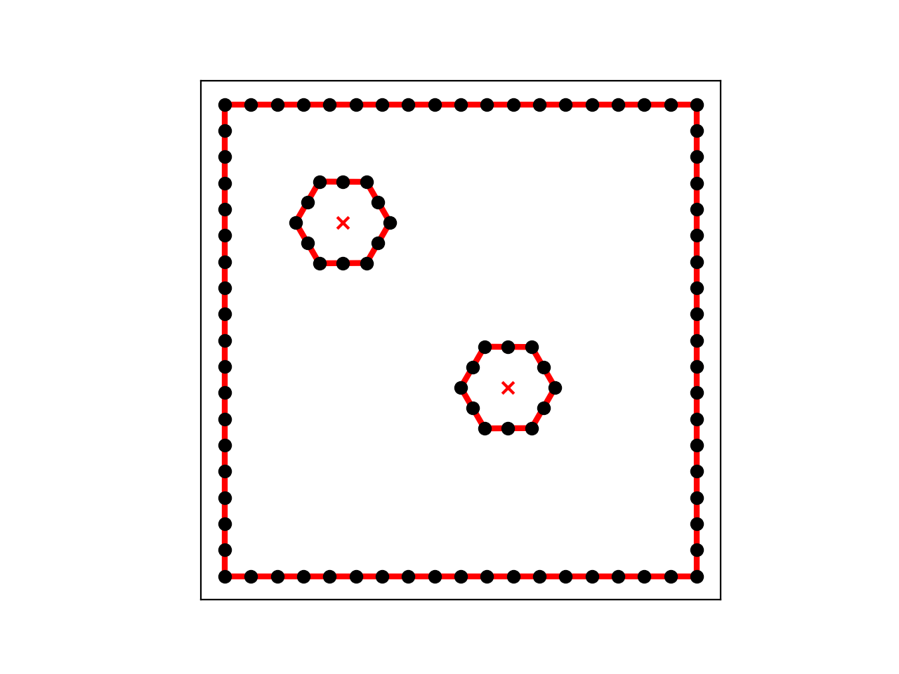
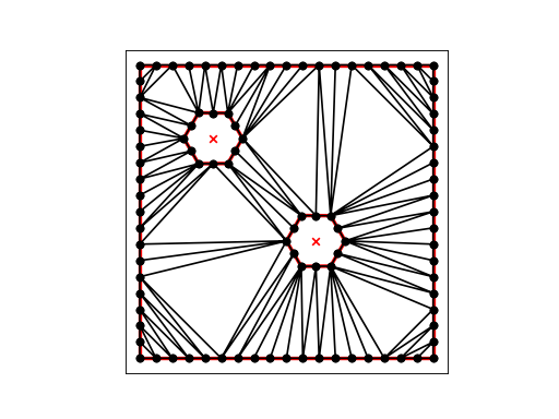
DOUBLE_HEX describes a unit square with two hexagonal holes. 72 points are listed on the outer boundary, and 12 on each of the holes. It is desired to create a nice looking mesh of about 500 nodes, and no additional nodes on the boundary segments.
(Source code, png, hires.png, pdf)

Our first command:
triangle -p double_hex.poly
requests that we triangulate the current points:
(Source code, png, hires.png, pdf)

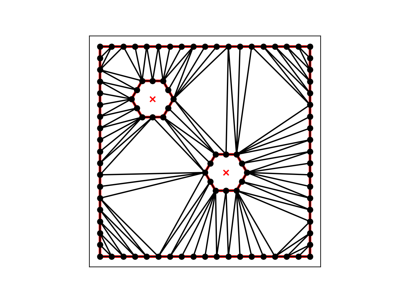
Our second command:
triangle -pqY -a0.0015 double_hex.1.poly
requests that we triangulate the current points, adding new nodes as necessary to make a nice mesh, with no triangle being larger than 0.0015 in area, and with no points added on boundary segments. We end up with 525 nodes and 956 elements:
(Source code, png, hires.png, pdf)

DOUBLE_HEX2
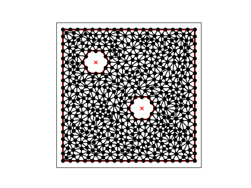
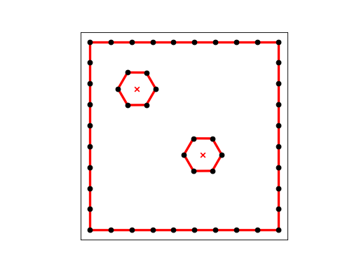
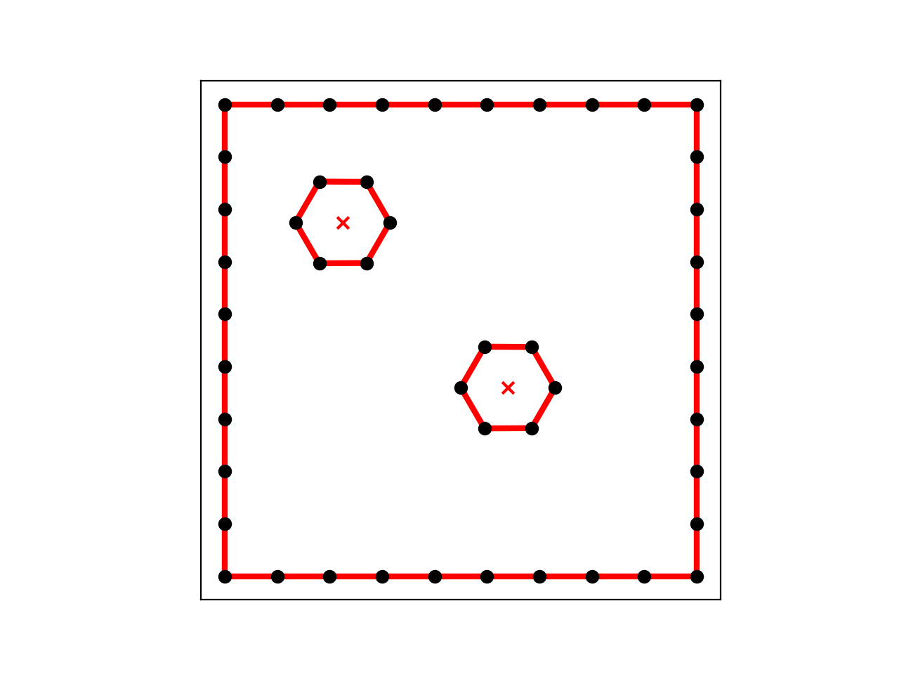
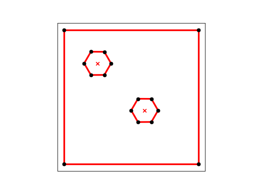
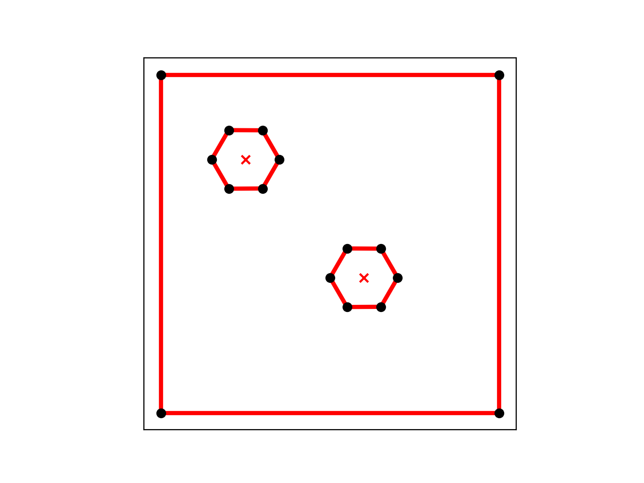
DOUBLE_HEX2 describes a unit square with two hexagonal holes. 36 points are listed on the outer boundary, and 6 on each of the holes. It is desired to create a nice looking mesh of about 235 elements, and no additional nodes on the boundary segments.
(Source code, png, hires.png, pdf)

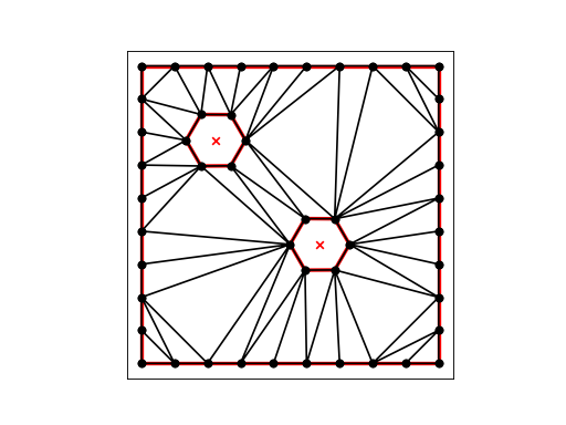
Our first command:
triangle -p double_hex2.poly
requests that we triangulate the current points:
(Source code, png, hires.png, pdf)
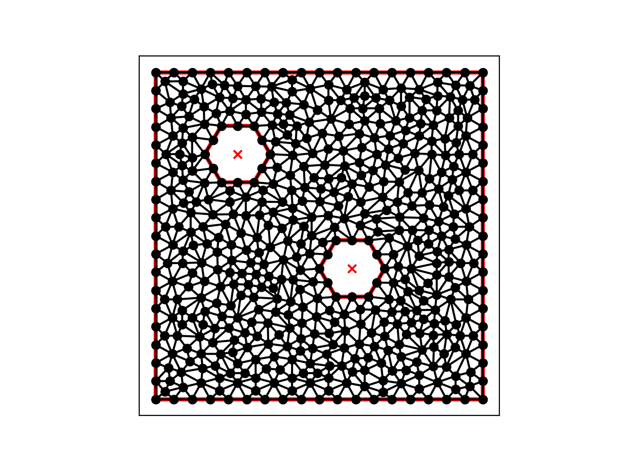
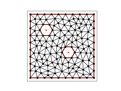
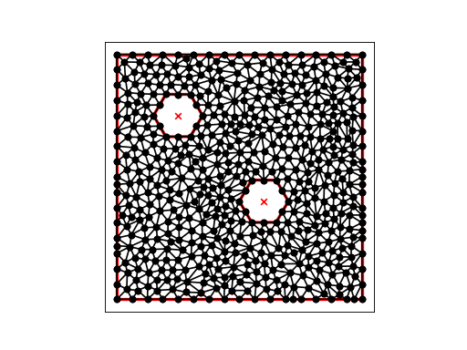
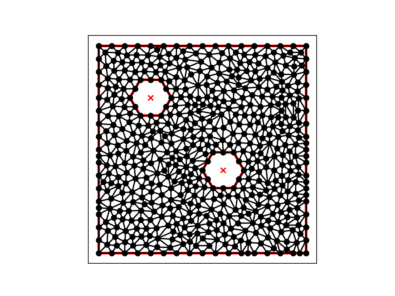
Our second command:
triangle -pqY -a0.0060 double_hex2.1.poly
requests that we triangulate the current points, adding new nodes as necessary to make a nice mesh, with no triangle being larger than 0.0060 in area, and with no points added on boundary segments. We end up with 141 nodes and 236 elements:
(Source code, png, hires.png, pdf)
DOUBLE_HEX3 describes a unit square with two hexagonal holes. 4 points are listed on the outer boundary, and 6 on each of the holes. We want triangle to triangulate this region.
(Source code, png, hires.png, pdf)

Our command:
triangle -pq -a0.0015 double_hex3.poly
requests that we triangulate the region, adding points as necessary so that no triangle has an area greater than 0.0015.
(Source code, png, hires.png, pdf)

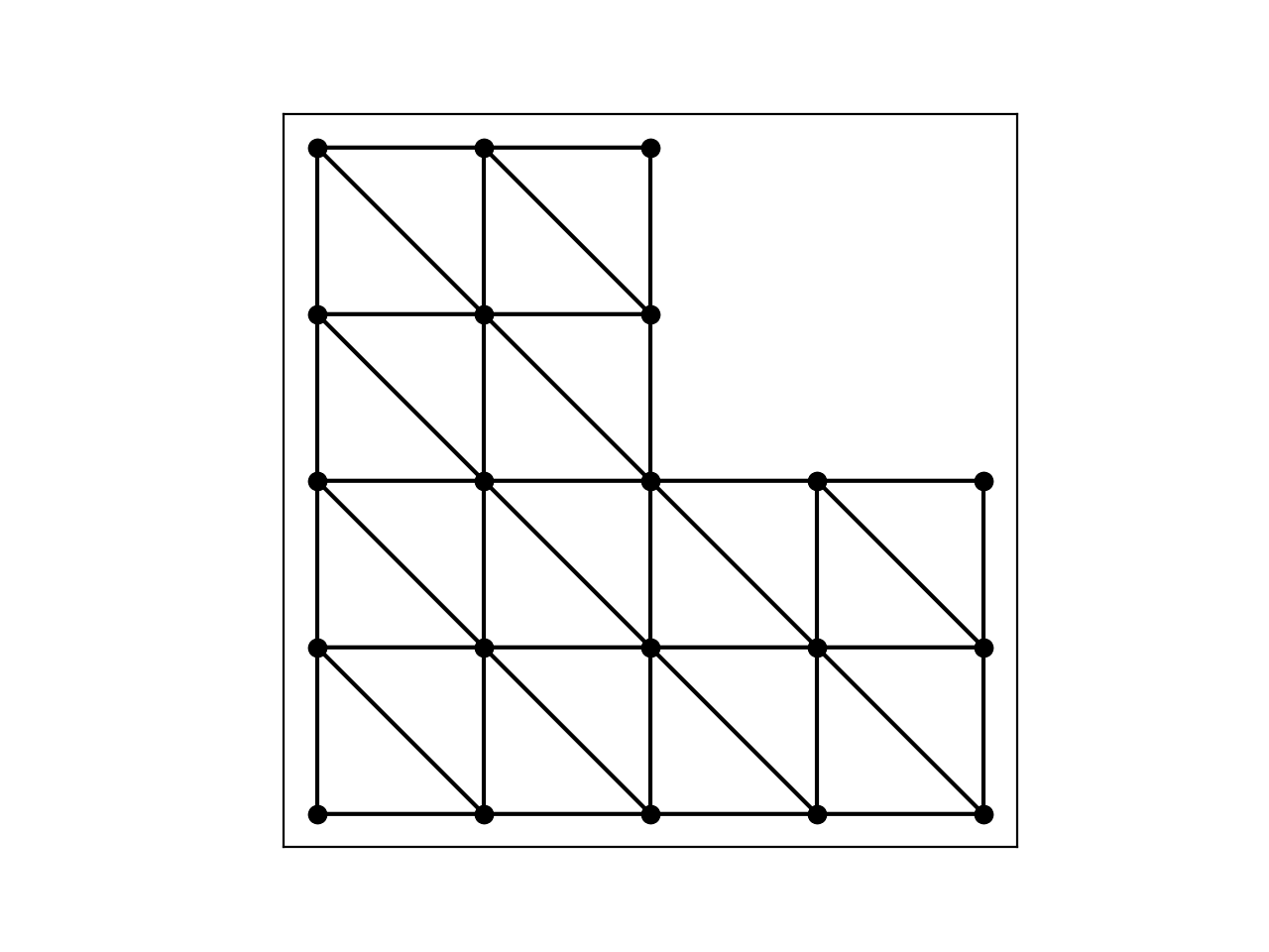
ELL
ELL is a triangulation of an L-shaped region, using a mesh of 21 nodes and 24 elements.
(Source code, png, hires.png, pdf)

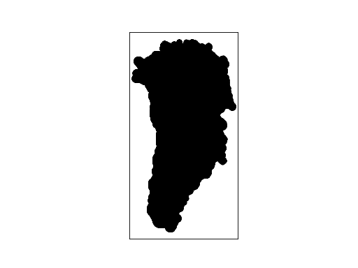
GREENLAND
GREENLAND is a triangulation of Greenland, using a graded (varying-size) mesh of 33,343 nodes and 64,125 elements. The resulting image is essentially a black blob the shape of Greenland. However, by modifying the code below, it is possible to see interesting details of the mesh.
(Source code, png, hires.png, pdf)

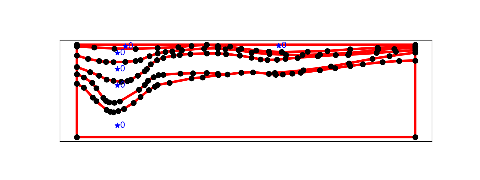
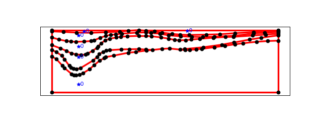
LA
LA is a POLY file containing information representing soil layers. The data includes points that are bounded by line segments defining the different layers. The intent is that certain layers will be triangulated with smaller area requirements.
(Source code, png, hires.png, pdf)
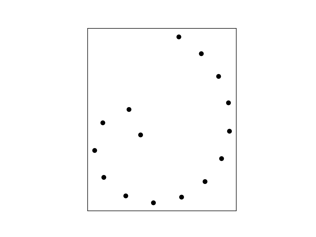
SPIRAL
SPIRAL is a node file containing points that form a spiral.
(Source code, png, hires.png, pdf)

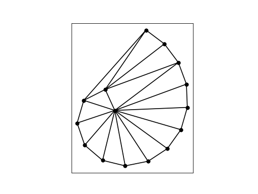
The command “triangle spiral” produces a Delaunay triangulation of the points, in the following node and element files:
(Source code, png, hires.png, pdf)
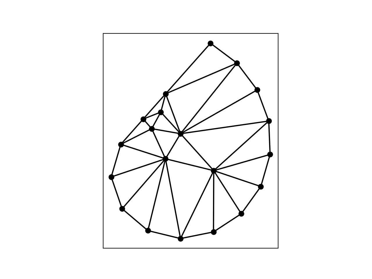
The command “triangle -q spiral” produces a Delaunay triangulation with no angle smaller than 20 degrees (the default). This is done by adding points as necessary: in the following node and element files:
(Source code, png, hires.png, pdf)
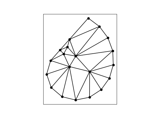
The command “triangle -q32.5 spiral” produces a Delaunay triangulation with no angle smaller than 32.5 degrees. This is done by adding points as necessary: in the following node and element files:
(Source code, png, hires.png, pdf)

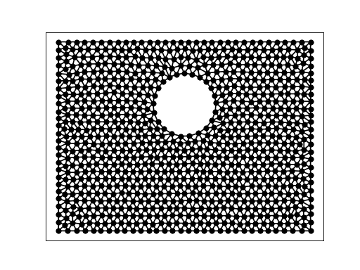
SQUARE_CIRCLE_HOLE
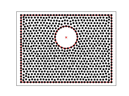
SQUARE_CIRCLE_HOLE is a planar straight line graph of a square region with an off center circular hole, and 826 points computed by a CVT calculation, prepared by Hua Fei.
(Source code, png, hires.png, pdf)

(Source code, png, hires.png, pdf)